
In this article, we present a parametric cellular-automata framework that makes it easy to build simulators and analysis tools for a wide range of automata.
The discussion is organized into two parts:
Cellular Automata Overview – a concise refresher on the core concepts.
The Parametric Framework – a walkthrough of the framework’s architecture and design choices.
I - Cellular Automata Overview
Cellular automata are mathematical models built on a finite population of cells. Each cell holds a state selected from a predefined set—finite for discrete automata and potentially continuous for analog variants. In the classic binary case, every cell is either ALIVE or DEAD. At each time step the system advances in lockstep: the new state of every cell is computed by applying a simple local rule that considers the current state of the cell and those of its neighbors. Repeated iterations of this rule generate successive “generations,” allowing intricate global patterns to emerge from straightforward local interactions.
Example
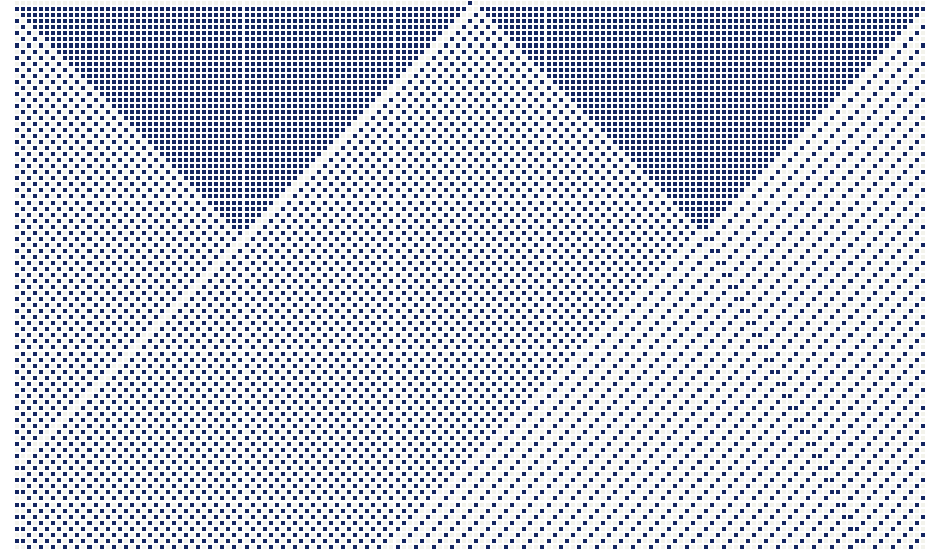
As an example, consider the one-dimensional cellular automaton governed by rule 163, illustrated in the figure below.

Each cell is either dead (gray) or alive (blue) and has exactly two neighbors—one to the left and one to the right. The rule determines a cell’s next state by examining this three-cell neighborhood (left neighbor, current cell, right neighbor). Because each of the three cells can be in one of two states, there are $2^3=8$ possible neighborhood configurations. Consequently, the rule is a Boolean function of three variables. Listing the outputs for the configurations in canonical order (from 111 to 000) produces the bit string 10100011, whose binary value corresponds to decimal 163—hence the name rule 163. Consequently, a one-dimensional binary-state automaton admits exactly $2^{2^3}=256$ distinct update rules—the full set of Boolean functions on three variables.
Starting with a single live cell at the grid’s center, successive iterations of rule 163 unfold into the intricate pattern illustrated below.
II- The Parametric Framework
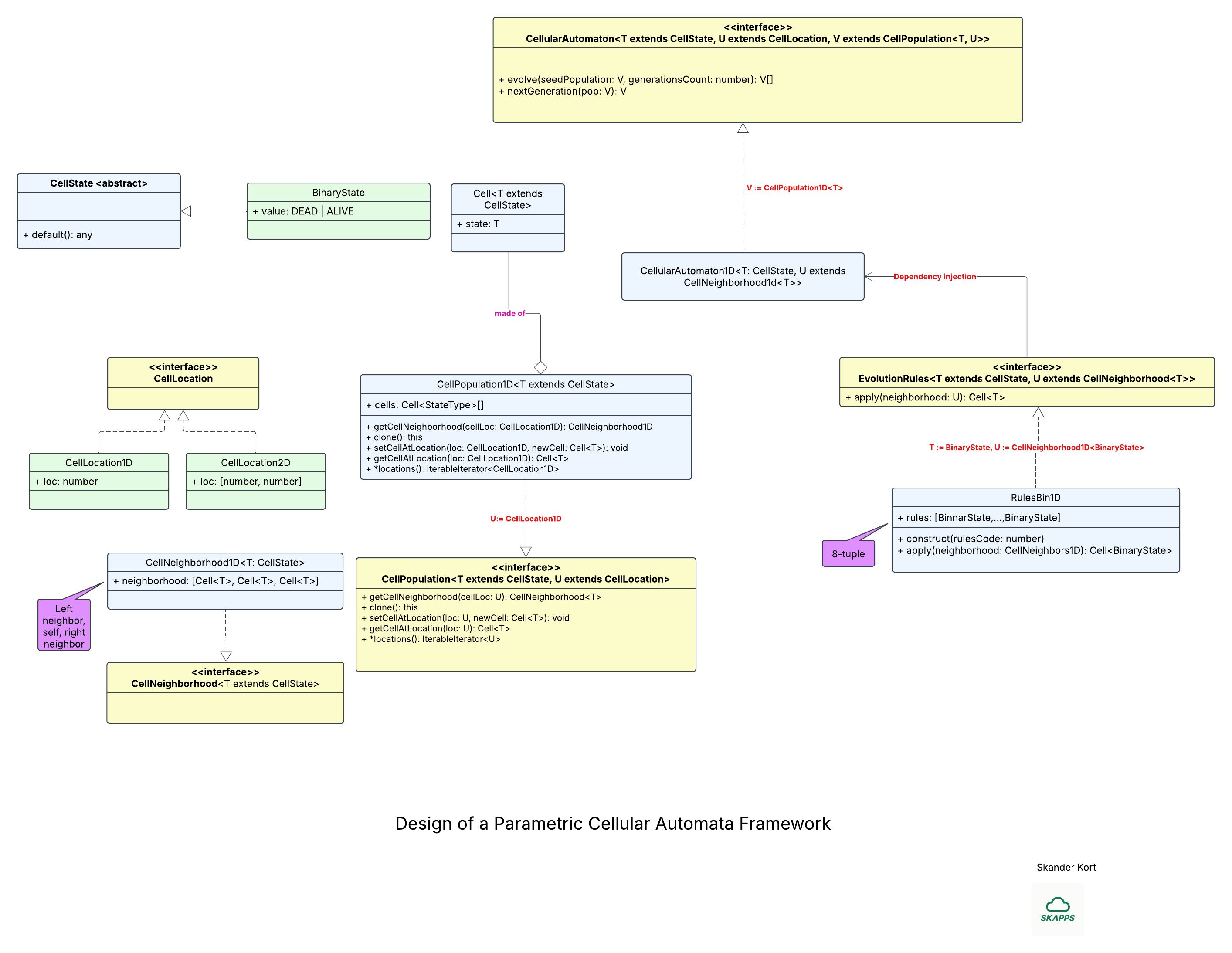
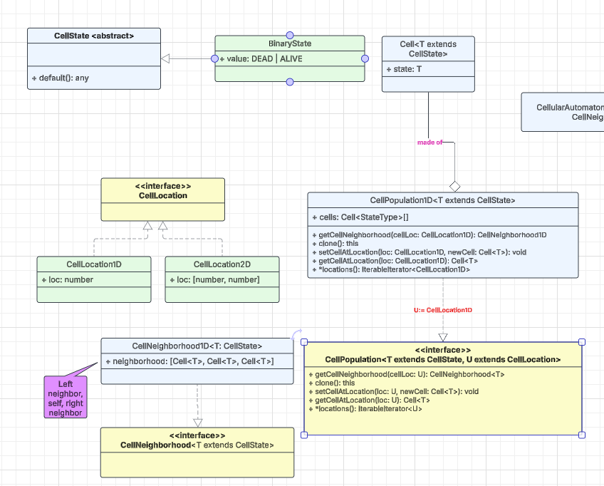
The framework’s architecture is illustrated in the diagram below, which we divide into two panels for clarity. The left panel highlights the low-level interfaces and implementation classes, while the right panel focuses on the higher-level abstractions that build on top of them.
This framework is built to accommodate cellular automata of any dimensionality whose cell states can take arbitrary values, whether discrete or continuous. The design grew out of a study of the diverse automata documented in Stephen Wolfram’s A New Kind of Science (NKS). Early on, we identified two key extension axes—cell-state space and grid dimensionality—and developed supporting abstractions such as neighborhoods and cell locations. These layers keep the core engine generic while letting developers plug in specific automaton rules with minimal friction.
We’ll start with the framework’s low-level interfaces and concrete classes. The diagram uses TypeScript-style notation, reflecting our choice of TypeScript for its expressive type system and its natural fit for building single-page applications.
A cell is represented by the polymorphic class Cell<T>, where the type parameter T extends the base class CellState. One concrete specialization, BinaryState, captures the classic two-valued case (ALIVE | DEAD) that dominates the cellular-automata literature; in TypeScript it can be modeled as either an enum or a union type.
For coordinate handling, the marker interface CellLocation provides a thin abstraction layer on which higher-level code can depend. In a two-dimensional grid, for example, a cell’s position is expressed as CellLocation2D, comprising its row and column indices.
The generic marker interface CellNeighborhood<T> abstracts the concept of a cell’s local neighborhood. In a one-dimensional population, the concrete implementation CellNeighborhood1D<T> captures this neighborhood as an ordered triple—⟨left, center, right⟩—matching the triplet used in the rule-163 example above.
The CellPopulation<T, U> interface represents the entire grid, abstracting away both dimensionality and state space. The type parameter T extends CellState captures the spectrum of allowable states, while U extends CellLocation encodes the coordinate system (1-D, 2-D, 3-D, and beyond). Its API exposes five core operations:
getCellNeighborhoodReturns the local neighborhood surrounding the specified cell.clone()Produces a copy—useful when computing the next generation.getCellAtLocationRetrieves the cell located at the given coordinates.setCellAtLocationUpdates the state of a specific cell.locations(): IteratableIterator<U>
Iterates over every coordinate in the population, agnostic to dimensionality.
A concrete subclass, CellPopulation1D<T>, implements this interface for one-dimensional grids whose cells can assume any state expressible by T.
Now, let's turn our attention to the high-level classes and interfaces in this design.
The EvolutionRules<T, U> interface abstracts the update logic that drives an automaton. In the familiar one-dimensional, binary-state case the rule table is fixed, but once you move to higher dimensions or richer state spaces the number of possible rules grows. Each rule operates on a neighborhood U that extends CellNeighborhood<T>, where T is any subtype of CellState. If that sounds abstract, the concrete class RulesBin1D anchors the concept: it implements the eight-bit rule family (e.g., rule 163) discussed earlier.
The CellularAutomator<T, U, V> interface represents a complete cellular-automaton engine and exposes two essential methods:
evolve()runs the automaton for a specified number of iterations, starting from an initial population.nextGeneration()advances the current population by a single step.
The incremental nextGeneration() call makes it easy to build a two-stage pipeline consisting of a CA (simulation) stage and a VIZ (visualization) stage. The CA stage streams one generation at a time to the VIZ stage, enabling smooth, real-time rendering—an approach that pays off when the update rule is computationally intensive.
A concrete implementation, CellularAutomaton1D, realizes this interface for one-dimensional populations with arbitrary state spaces. Notice that the evolution rule is supplied via dependency injection, keeping the core automaton decoupled from any specific rule logic.
Because the interface is fully parameterized, a single, well-designed implementation of CellularAutomaton can typically support grids of any dimensionality and cells drawn from any state space