Analyzing the Upper Confidence Bound Algorithm

This article focuses on evaluating the implementation of the Upper Confidence Bound (UCB) algorithm discussed herein. The evaluation is conducted using a single dataset provided by Super Data Science.

The Dataset

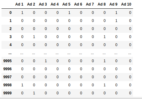
The dataset is a matrix with $10,000$ rows and $10$ columns. Each row represents a request made to an online ad server to display an advertisement. The ad server has a catalog of $10$ ads: ${Ad_1, \ldots, Ad_{10}}$. The value in cell $(i, j)$ is 1 if and only if ad $Ad_j$ would be clicked when displayed to a user visiting the website; otherwise, the value is 0. Importantly, this information is unknown to the ad server at the time of ad selection.

The ad server aims to select an ad that is most likely to be clicked, using historical data to make informed decisions. This approach seeks to maximize revenue for publishers (website owners) while optimizing reach for advertisers.

The problem can be modeled as a multi-armed bandit game, where:

• Each advertisement represents an arm of the bandit, yielding a reward of 1 if the corresponding ad is clicked.
• Each ad request event corresponds to a round of the game.
• The ad server acts as the player in this game, tasked with selecting the optimal arm to maximize rewards.

Initializing and Running UCB

Let’s now set up the UCB algorithm and put it to the test by playing the multi-armed bandit game using the dataset described earlier. To begin, we’ll import all the necessary Python libraries required for this analysis, laying the groundwork for our implementation.

import numpy as np
import matplotlib.pyplot as plt
from matplotlib import colors
import pandas as pd
import math
from ucb import UpperConfidenceBound

Loading the dataset is made easy, thanks to Pandas library:

dataset = pd.read_csv('ad_server.csv') 

Finally, we create an instance of the UpperConfidenceBound class and initiate the game, or reinforcement learning process, by calling its learn() method.

n_rounds = 10000
training_set = dataset[:n_rounds + 1]
ucb = UpperConfidenceBound(training_set.values)
ucb.learn()

Total Reward

The objective of the ad server is to maximize revenue, which translates to maximizing the total reward by the end of the multi-armed bandit game. Upon examining the dataset, we notice rows where all columns contain zeroes (like rows $2$ and $4$ in the figure above). This means that for these specific ad request events, regardless of which ad is served, no clicks will occur from the ad impressions.

So, first, let's calculate the optimum reward one hopes to reach. This is equivalent to counting the rows where all columns are zeroes.

rows_with_all_zeros = dataset[(dataset == 0).all(axis=1)].shape[0]
print(f"Number of rows with all zeros: {rows_with_all_zeros}")
optimum_reward = n_rounds - rows_with_all_zeros
print(f"The optmum reward is {optimum_reward}")

In this dataset, the optimum reward is $7424$. We define the efficiency of a multi-armed bandit strategy as: $$efficiency = \frac{total\_reward(strategy)}{optimum\_reward}$$

The code snippet below, calculates the total reward and the efficiency of UCB:

total_reward = ucb.total_reward()
efficiency = round(total_reward * 100.0 / optimum_reward)

The UCB algorithm achieved a total reward of $2211$, which is only $30\%$ of the optimal reward. This indicates significant potential for improvement.

Most Served Ad

In this section, I will demonstrate how often each advertisement was served. Recall the array UpperConfidenceBound.selected_candidates(). To visualize this, we can simply plot the array as a histogram using the code provided below.

freqs, bins, patches = plt.hist(ucb.selected_candidates())
print(f"Frequency of each ad: {','.join(map(lambda fr: str(int(fr)), freqs))}")
plt.xlabel('Ad index')
plt.ylabel('Impressions')
plt.title('Number of times an ad is displayed')
norm_freqs = freqs / freqs.max() 
norm = colors.Normalize(norm_freqs.min(), norm_freqs.max())
print(norm)
for thisfrac, thispatch in zip(norm_freqs, patches):
    color = plt.cm.cividis(norm(thisfrac))
    thispatch.set_facecolor(color)
plt.show()

This produces the histogram shown below.

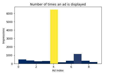
The diagram reveals that $Ad_5$ was the most frequently displayed advertisement, with $Ad_8$ being the second most served.

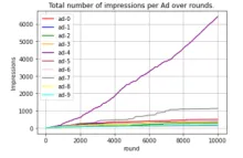
Analyzing the Behavior of UCB Over Time

In this section, we aim to gain insights into the behavior of the UCB algorithm over time. Specifically, we will examine when UCB begins recognizing $Ad_5$ as the best-performing ad. Additionally, we will investigate whether UCB eventually stops selecting certain ads after a certain number of rounds or if it continues exploring all ads to maintain learning opportunities.

To conduct a more granular analysis, we need to track the number of impressions each ad receives over time, rather than just the cumulative impressions. This can be achieved by introducing a new state variable in the UpperConfidenceBound class called __n_selected_round. This variable is a two-dimensional array where rows represent rounds, and columns correspond to ads. Item __n_selected_round[round_idx][ad_idx] represents the number of impressions received by ad ad_idx up to round round_idx. 

The implementation of UpperConfidenceBound is updated accordingly.

def __reset_state(self):
        self.__n_selected_round: List[List[int]] = np.zeros(self.__rewards_by_round.shape, dtype=int)
        ...
        
def __select_candidate(self, candidate_idx: int, round_idx: int):
        self.__n_selected[candidate_idx] += 1
        self.__n_selected_round[round_idx] = self.__n_selected

Next, let’s visualize how the number of impressions evolves for each ad over time. To do this, we will use the following Python code snippet.

n_selected_round = ucb.get_number_selected_round()
colors = ["red", "blue", "green", "orange", "purple", "brown", "pink", "gray", "yellow", "cyan"]
for i in range(0, 10):
    plt.plot(range(0, n_rounds), n_selected_round[:, i], color=colors[i], label=f'ad-{i}')
plt.xlabel('round')
plt.ylabel('Impressions')
plt.title('Total number of impressions per Ad over rounds.')
plt.grid()
plt.legend()
plt.show()

Executing this code generates the following plot.

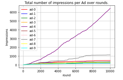
$Ad_5$ is selected far more frequently than any other ad, with this behavior emerging around round 1000. While other ads continue to be selected in later rounds, some appear to plateau toward the end of the game, indicating a decrease in selection frequency. To better understand how UCB handles non-optimal ads, let's exclude the curve for $Ad_5$ from the figure above.

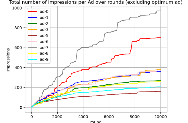
This figure reveals that some ads stop being selected shortly after round 8000—for example, ad-5, which UCB identifies as the least-performing ad. Meanwhile, others, like ad-7, the second-best-performing ad, continue to be selected until the end of the game.