The Exploration-Exploitation Balance: The Epsilon-Greedy Approach in Multi-Armed Bandits

In this article, I will explore the balance between exploration and exploitation, a key concept in reinforcement learning and optimization problems. To illustrate this, I will use the multi-armed bandit problem as an example. I will also explain how the epsilon-greedy strategy effectively manages this balance.

I- The Exploration-Exploitation Balance 

In the article Comparison of Three Multi-Armed Bandit (MAB) Strategies, I evaluated the efficiency of three MAB algorithms: Random Selection, Maximum Average Reward (MAR), and Upper Confidence Bound (UCB). The results showed that the Random Selection algorithm achieved an efficiency of 17%, serving as the baseline. UCB emerged as the most effective arm selection strategy with an efficiency of 30%. In contrast, MAR proved to be the least effective, with an efficiency of just 7%, falling below even the baseline Random Selection algorithm.

An initial investigation revealed that the MAR algorithm quickly settles on the arm with the highest average reward during the MAB warm-up phase. This behavior makes MAR a purely exploitative strategy, as it relies solely on its current belief without seeking new information. However, effective reinforcement learning and optimization algorithms should avoid prematurely converging to a seemingly optimal solution, as this often leads to getting stuck in a local optimum. To avoid this, they should occasionally explore alternative solutions to ensure they find the true global optimum.

In the context of MAB, repeatedly selecting the arm identified as the best so far is known as exploitation. Conversely, choosing an arm other than the current best is called exploration. Exploration enables MAB strategies to discover potentially better arms throughout the game, allowing them to escape local optima and ultimately achieve higher rewards.

Both MAR and UCB belong to a category of algorithms known as greedy deterministic (or non-stochastic) algorithms. These strategies calculate a score for each arm in a given round and select the arm that maximizes this score. However, despite their similar approach, UCB outperforms MAR. Why is this the case? To understand this discrepancy, let's examine the scoring mechanisms used by each MAB strategy.

Recall that in the MAR strategy, the score assigned to arm $i$ at round $n$ is  $$ \bar{r}_i(n) = \frac{R_i(n)}{N_i(n)}$$ which represents the average reward yielded by arm $i$ up to round $n$. This score makes MAR purely expoitative. 

In contrast, UCB assigns a score to arm $i$ at round $n$ that combines two  components: the average reward obtained from arm $i$ and the upper bound of the confidence interval for the reward of that arm. This confidence interval reflects the uncertainty about the true value of the reward: $$ \bar{r}_i(n)  + \Delta_i(n)$$ where $$ \Delta_i(n) = \sqrt{\frac{3}{2}\frac{\log(n)}{N_i(n)}}$$ Intuitively, the term $Delta_i(n)$ increases the score of arms that have been pulled infrequently (i.e. have a low number of pulls $N_i(n)$) up to round $n$. This boost incentivizes exploration by encouraging the selection of less-tested arms, thereby reducing uncertainty about their potential rewards.

I often refer to  term $ \Delta_i(n)$ in the UCB's arm score formula a regulization term. In machine learning, regularization is commonly used to prevent overfitting, which occurs when a model becomes overly tailored to the training data, leading to poor generalization on unseen data. Similarly, in UCB, regularization helps balance exploration and exploitation, preventing the algorithm from prematurely committing to arms with seemingly high average rewards. Let's examine how regularization operates within the UCB strategy.

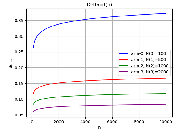
Consider four hypothetical arms indexed from $0$ to $3$, which have been pulled 100, 500, 1000, and 2000 times, respectively. The figure below illustrates how $ \Delta_i(n)$ term evolves as a function of the round index. This term grows at a moderate pace, preventing UCB from exploring alternative arms too aggressively. As a result, the score of the least-pulled arm (i.e. arm-0) receives a boost of approximately $0.4$ in the later rounds. In contrast, the most-pulled arm's score ( (i.e. arm-3) ) increases by only about $0.08$ towards the end of the game. In other words, an arm will still be selected by UCB if its average reward is within 0.32 of the best-performing arm, ensuring a balanced approach between exploration and exploitation.

II- Agnostic Exploration: The Epsilon-Greedy Approach

In Section I, we examined how UCB explores alternative arms using information gathered throughout multiple MAB games (also known as episodes). However, exploration can also be approached in an agnostic manner, independent of any knowledge gained during an episode. This type of exploration is purely random, earning it the name agnostic exploration. Greedy algorithms that incorporate this randomness are known as epsilon-greedy strategies.

The concept behind epsilon-greedy MABs is straightforward. Most of the time, the strategy selects an arm based on a calculated score. However, at random intervals, it chooses to explore by pulling a different, randomly selected arm. The frequency of these exploratory moves is controlled by the parameter $\epsilon$ commonly referred to as the learning rate in epsilon-greedy algorithms. 

Let's now integrate epsilon-greedy exploration into our MAB framework.

III- Integrating Epsilon-Greedy Exploration Into MAB Framework

Integrating epsilon-greedy into our MAB framework involves two key steps. First, we inject the exploration rate parameter ($\epsilon$) into the constructor of the MultiArmedBandit class:

class MultiArmedBandit:
    def __init__(self, arm_selector: ArmSelection, rewards_matrix: List[List[int]], eps_greedy_rate: float = 0.0):
    ...
    self.__eps_greedy_rate = eps_greedy_rate

Next, the __select_pull_arms() method is modified to allow for random exploration of arms.

def __select_pull_arms(self) -> None:
        """
        Selects an arm per ArmSelection strategy, then pulls it.
        """
        for _ in range(self.__game_state.current_round, self.__max_rounds):
            rnd = random.random()

            if rnd <= self.__eps_greedy_rate:
                selected_arms_idx = random.randrange(self.__num_arms)
            else:
                selected_arms_idx = self.__arm_selector.select(copy.deepcopy(self.__game_state))

            self.__pull_single_arm(selected_arms_idx)

A random number rnd is  generated from a uniform distribution between $0$ and $1$. If rnd is less than $\epsilon$, then the algorithm explores by randomly selecting an arm. Otherwise, it exploits by delegating the arm selection to the existing ArmSelection strategy.

With epsilon-greedy exploration integrated into our MAB framework, we can now investigate whether it enhances the performance of the existing MAB strategies. This evaluation will be the focus of the next section.

 IV- Evaluation of Epsilon-Greedy MABs

In this section, we will examine the performance of two MAB strategies: MAR and UCB. Specifically, we will evaluate the efficiency of each strategy using different values of $\epsilon$. o conduct this analysis, two utility functions are required.

1- Utility functions

First, we need a function that enables us to run a multi-armed bandit with various values of $\epsilon$ This function, named grid_search(), evaluates the efficiency of the MAB strategy for each value of $\epsilon$$\epsilon$ and returns the corresponding performance metrics.

def grid_search(armSelector: ArmSelection, rewards_matrix: List[List[int]], 
                epsilon_range: np.ndarray, num_rounds: int) -> List[float]:
    print('Started running bandit...')
    efficiency = []

    for epsilon in epsilon_range:
        print(f'epsilon = {epsilon}')
        mab = MultiArmedBandit(armSelector, rewards_matrix, epsilon)
        mab.play(num_rounds)
        efficiency.append(mab.get_efficiency())
       
    print('Done running bandit.')
    return efficiency

Next, we extend the MabPlotting class introduced in the MAB evaluation article by adding a new method. This method visualizes MAB efficiency as a function of $\epsilon$

@staticmethod
def plot_efficiency_epsilon(plotter, epsilon: np.ndarray, efficiency: List[float]) -> None:
    plotter.plot(epsilon, efficiency)
    plotter.xlabel('epsilon')
    plotter.ylabel('efficiency')
    plotter.title('MAB efficiency v.s. epsilon greedy learning rate')
    plotter.grid()
    plotter.show()    

2- Evaluation of MAR

Let's run a grid search on MAR with various values of $\epsilon$ and collect the efficiency of each run.

import numpy as np

num_rounds = 10000
epsilon_range = np.arange(0, 1.05, 0.05)

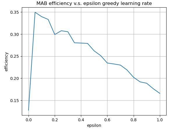
avg_mab_efficiency = grid_search(MaxAverageRewardSelector(), dataset.values, epsilon_range, num_rounds) 

 Let’s now visualize how the efficiency of each MAR run varies with different values of $\epsilon$. The figure below illustrates that the efficiency of MAR increases sharply for small values of $\epsilon$$\epsilon$ reaching a peak of $0.34$. Beyond this point, efficiency gradually declines, eventually converging to $0.17$, the efficiency level of a purely random strategy. The maximum efficiency is reached at $\epsilon = 0.1$.

3- Evaluation of UCB

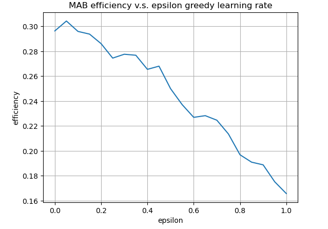
We conduct a similar analysis for UCB with various values of $\epsilon$. The curve below shows that epsilon-greedy does not combine well with UCB. 

V- Concluding Remarks

Introducing random exploration with a learning rate of 0.1 significantly enhances the efficiency of the Maximum Average Reward (MAR) MAB strategy, boosting it from 7% to 34%—a remarkable improvement. However, for Upper Confidence Bound (UCB), the addition of random exploration leads to a decline in efficiency. This is because the randomness interferes with UCB's inherently informed exploration mechanism. Notably, MAR with an $\epsilon$ of 0.1 outperforms UCB, making it the most effective MAB strategy among those studied, given the dataset at hand.