Stochastic Multi-armed Bandit - Thompson Sampling With Beta Distribution

We have previously explored two multi-armed bandit (MAB) strategies: Maximum Average Reward (MAR) and Upper Confidence Bound (UCB). Both approaches rely on the observed average reward to determine which arm to pull next, using a deterministic scoring mechanism for decision-making. However, MAR performs poorly because it lacks an exploration component, failing to consider potentially better arms throughout the game. In contrast, UCB incorporates an exploration bonus, allowing it to occasionally test alternative arms, which improves its overall efficiency. Additionally, we examined the epsilon-greedy strategy, an exploration method that operates independently of the primary MAB strategy. When combined with other MAB techniques, epsilon-greedy facilitates periodic exploration of alternative arms.

In this article, we introduce a different class of MAB algorithms known as stochastic strategies, which integrate exploration in a probabilistic manner. Specifically, we focus on Thompson Sampling with a Beta Distribution (TSB), a widely used Bayesian approach to the exploration-exploitation tradeoff. In a future post, we will explore Thompson Sampling with a Gaussian Distribution, another variant of this method.

I- Thompson Sampling With Beta Distribution

Thompson Sampling with a Beta Distribution (TSB) is particularly suited for scenarios where the reward associated with each arm in a multi-armed bandit (MAB) problem is binary. A typical example is in digital marketing, where each arm represents a notification sent to users via a mobile app, and a reward is received if a user takes a desired action—such as making a purchase—in response to the notification.

Without loss of generality, we assume that rewards take values of either 0 (no reward) or 1 (reward received). In TSB, each arm is modeled as a binary random variable, where its success probability is unknown and must be learned over time. To achieve this, we assume that each arm’s success probability follows a Beta distribution, which serves as a prior belief that gets updated as more data is observed. The Beta distribution is defined by the following probability density function: $$f(x, \alpha, \beta) = \frac{x^{\alpha - 1}(1-x)^{\alpha - 1}}{B(\alpha, \beta)}$$ where:

• $\alpha$ is number of observed successes plus one.
• $\beta$ is the number of observed failures plus one.
• $B(\alpha, \beta)$ is a normalization constant.

Let us explore how  the shape of Beta distribution varies with different values of parameters $\alpha$ and $\beta$. This will provide insight into how Thompson Sampling with a Beta Distribution adapts its decision-making process based on observed rewards

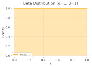
When $\alpha=\beta=1$, meaning no observations have been made yet, the algorithm lacks any prior knowledge to inform its decisions. In other words, this represents a state of maximum entropy, where all outcomes are equally likely. In this case, the Beta distribution simplifies to a uniform distribution over the interval $[0, 1]$ , meaning any value within this range is sampled with equal probability.

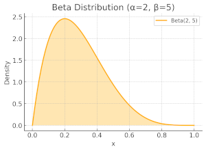
Now, consider the case where $\alpha=2$ and $\beta=5$, meaning that one success has been observed compared to four failures. Beta distribution becomes skewed towards zero, reflecting the algorithm's current belief that the probability of success is relatively low. Consequently, lower values are more likely to be sampled.

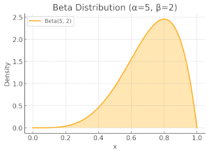
Symmetrically, when $\alpha=5$ and $\beta=2$, the distribution becomes skewed towards one.

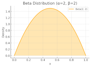
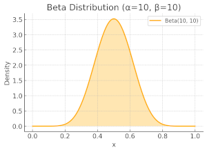
Now, let's examine two scenarios: first, when $\alpha=\beta=2$, and then when  $\alpha=\beta=10$. In both cases, the Beta distribution forms a symmetric, bell-shaped curve centred around 0.5, indicating that the most likely sampled value is 0.5. This suggests that arms are selected with roughly equal probabilities. However, there is a key difference: the distribution in the $\alpha=\beta=10$ case is more concentrated around 0.5, meaning the probability mass is less spread out compared to the $\alpha=\beta=2$. This reflects a lower standard deviation, signifying increased confidence in the estimated probability of success. In other words, as more observations are collected, our uncertainty decreases, entropy is reduced, and the algorithm becomes more certain about which arms are optimal.

II- Implementation of Thompson Sampling With Beta Distribution

Thompson Sampling with a Beta Distribution seamlessly integrates into our previously described MAB framework as a concrete implementation of the ArmSelection interface.

    class ThomsonBetaSampling(ArmSelection):
    """
    Thompson Sampling for multi-armed bandits with binary rewards assumes that each arm follows a Beta distribution. 
    As the bandit game progresses, the algorithm continuously updates the parameters of the Beta distribution.
    """
    def select(self, game_state: GameState) -> int:
        best_arm: Optional[int] = None
        max_theta = 0.0
        for candidate_arm in range(game_state.num_arms):
            alpha = game_state.arms_rewards[candidate_arm] # Number of successful pulls (ones)
            beta = game_state.num_arms_pulls[candidate_arm] - alpha # Number of failed pulls (zeroes)
            theta = random.betavariate(alpha + 1, beta + 1)
            if theta >= max_theta:
                max_theta = theta
                best_arm = candidate_arm
        return best_arm  

The select() method iterates over all candidate arms and performs the following steps:

1. For each arm, it retrieves the observed number of successes ($\alpha$) and failures ($\beta$) from the current GameState.
2. It then samples a random value $\theta$ from a Beta distribution using the random.betavariate() function.
3. Finally, it selects the arm corresponding to the maximum value of  $\theta$, ensuring a balance between exploration and exploitation.

III- Evaluation of Thompson Sampling with Beta Distribution

In this section, we compare the efficiency of TSB against previously discussed MAB algorithms. To ensure consistency, we use the ads dataset introduced in the comparative study article.

First, we initialize an MAB instance using TSB.

thp_beta_mab = MultiArmedBandit(ThomsonBetaSampling(), dataset.values)

Using code snippets similar to those presented in the UCB analysis article, we compute the efficiency of TSB and generate relevant visualizations. For brevity, we present only the final results here.

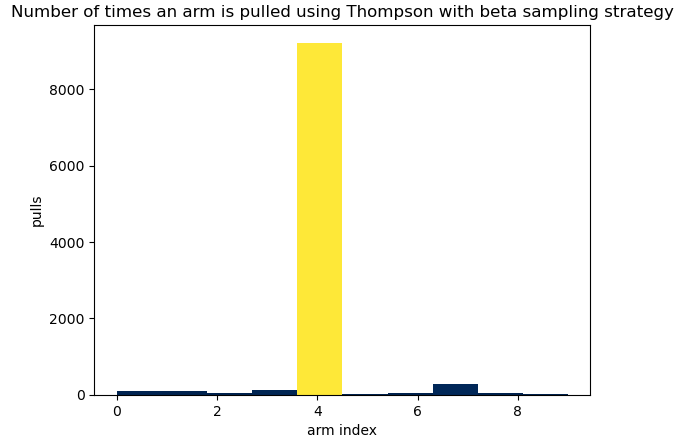
TSB achieves an efficiency of 35%, making it the best-performing MAB strategy so far. In comparison, MAR with epsilon-greedy (with $\epsilon=01$) attains 34% efficiency, while UCB lags behind at 30% efficiency, given the dataset at hand.

TSB, like epsilon-greedy MAR and UCB, tends to favor arm-4 more frequently. However, the stochastic nature of Thompson Sampling leads to a more aggressive exploitation of this arm compared to the deterministic approach of UCB. This probabilistic selection mechanism allows TSB to dynamically balance exploration and exploitation, adapting more effectively to the observed reward distributions.

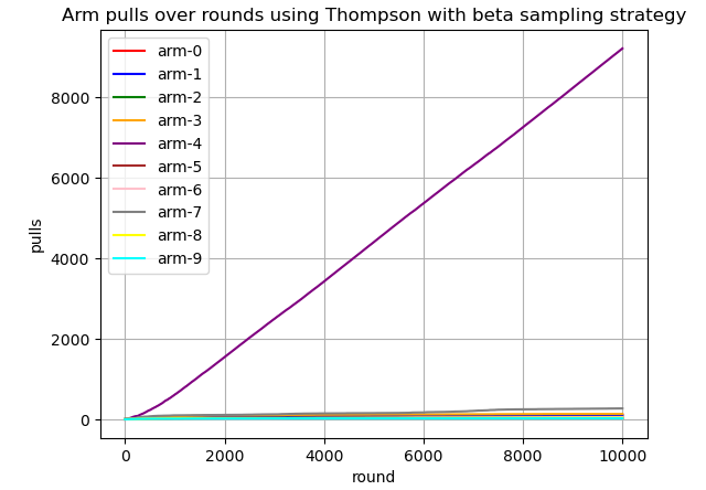
Finally, the visulization below depicts how TSB pulls arms over time.

  IV- Concluding Remarks

In this article, we introduced a stochastic algorithm for solving the multi-armed bandit problem: Thompson Sampling with a Beta Distribution. We explored both the theoretical foundations and the intuition behind TSB before integrating it into our MAB framework.

Our experimental results demonstrated that TSB’s adaptive, probabilistic exploration strategy enabled it to slightly outperform epsilon-greedy MAR, which relies on purely random exploration, and UCB, which follows a deterministic approach. This highlights the effectiveness of TSB in dynamically balancing exploration and exploitation, leading to improved decision-making in MAB scenarios.